SqueezeDet: Deep Learning for Object Detection
Why bother writing this post?
Often, examples you see around computer vision and deep learning is about classification. Those class of problems are asking what do you see in the image? Object detection is another class of problems that ask where in the image do you see it?
Classification answers
whatand Object Detection answerswhere.
Object detection has been making great advancement in recent years. The hello world of object detection would be using HOG features combined with a classifier like SVM and using sliding windows to make predictions at different patches of the image. This complex pipeline has a major drawback!
Cons:
- Computationally expensive.
- Multiple step pipeline.
- Requires feature engineering.
- Each step in the pipeline has parameters that need to be tuned individually, but can only be tested together. Resulting in a complex trial and error process that is not unified.
- Not realtime.
Pros:
- Easy to implement, relatively speaking…
Speed becomes a major concern when we are thinking of running these models on the edge (IoT, mobile, cars). For example, a car needs to detect where other cars, people and bikes are to name a few; I could go on… puppies, kittens… you get the idea. The major motivation for me is the need for speed given the constraints that edge computes have; we need compact models that can make quick predictions and are energy efficient.
The SqueezeDet Model
The latest in object detection is to use a convolutional neural network (CNN) that outputs a regression to predict the bounding boxes. This post is about SqueezeDet. I got interested because they used one of my favorite cnn, SqueezeNet! You can read my last post on SqueezeNet if you haven’t yet. To be fair SqueezeDet is pretty much just the YOLO model that uses a SqueezeNet.
Highlevel SqueezeDet
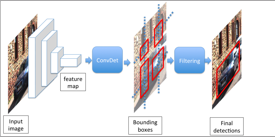
Inspired by YOLO, SqueezeDet is a single stage detection pipeline that does region proposal and classification by one single network. The cnn first extracts feature maps from the input image and feeds it to the ConvDet layer. ConvDet takes the feature maps, overlays them with a WxH grid and at each cell computes K pre-computed bounding boxes called anchors. Each bounding box has the following:
- Four scalars (x, y, w, h)
- A confidence score ( Pr(Object)xIOU )
Cconditional classes
Hence SqueezeDet has a fixed output of WxHxK(4+1+C).
The final step is to use non max suppression aka NMS to filter the bounding boxes to make the final predictions.
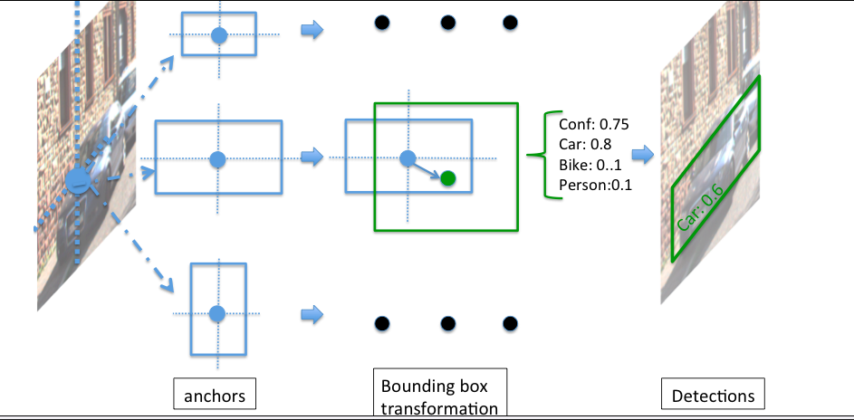
The networks regresses and learns how to transform the highest probably bounding box for the prediction. Since there are bounding boxes being generated at each cells of the grid, the top N bounding boxes sorted by the confidence score are kept as the predictions.
The Composite Loss function
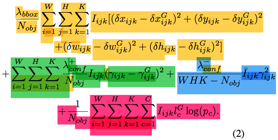
The figure above is the four part loss function that makes this entire model possible. Don’t get intimidated by it; let’s take it apart and see how it fits together. Each loss function is described below and highlighted:
Note: The yellow that bleed into the blue loss function is actually suppose to be blue, sorry!
- Yellow: Regression of the scalars for the anchors
- Green: The confidence score regression which uses IOU of ground and predicted bounding boxes.
- Blue: Penalize anchors that are not responsible for detection by dropping their confidence score.
- Pink: The cross entropy.
Using SqueezeDet
The authors of the paper did implement the model via TensorFlow! Go check it out on github https://github.com/BichenWuUCB/squeezeDet
Thresholding SqueezeDet
You have to tweak how confident or doubtful you want the model to be; the predictions are centered around K bounding boxes at each cell. So we have to use the top N bouding boxes, sorted by confidence score and then you can do additional thresholding on the class conditional probability score.
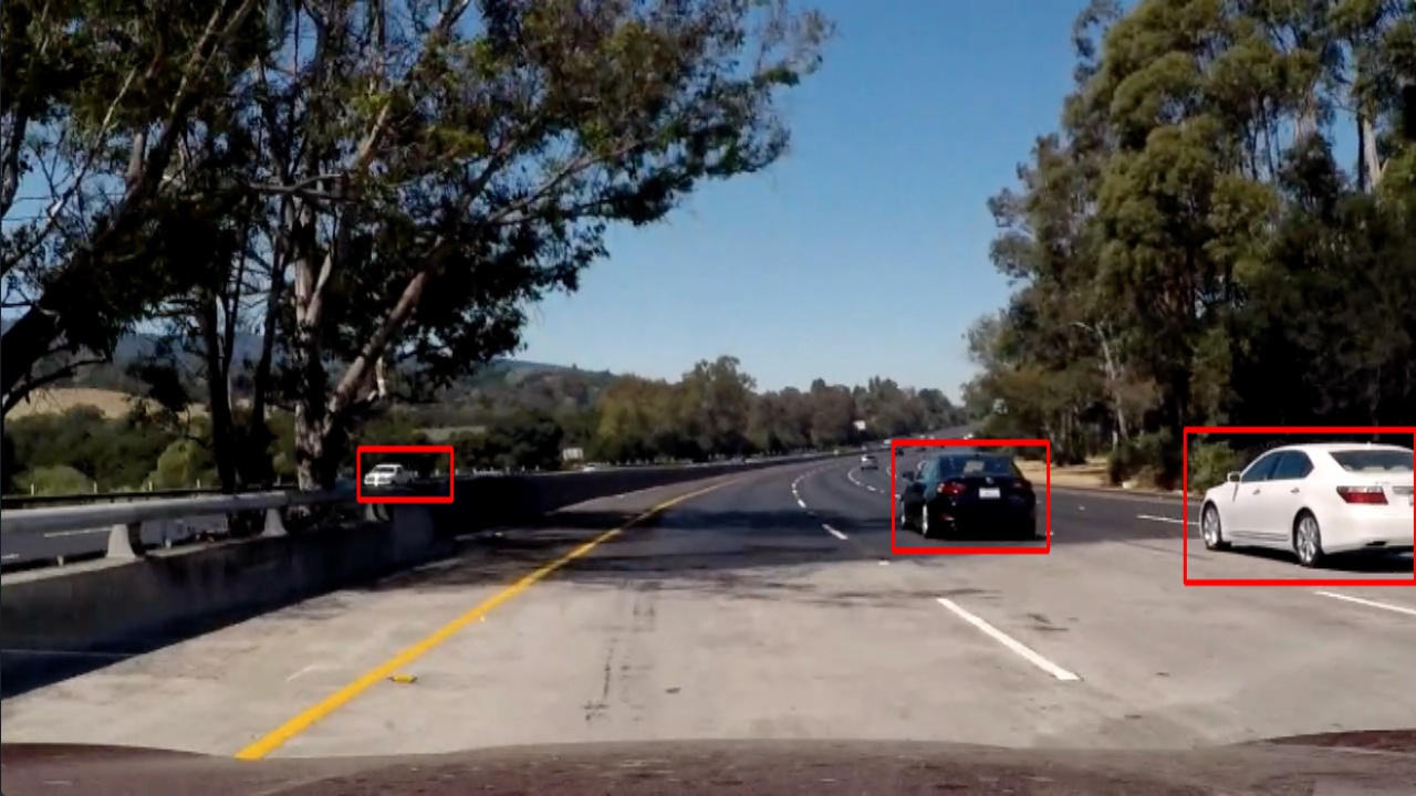
Here is an example of a recent project I did where I tweak the params:
Like the paper:
N = 64
The image below shows mc.PLOT_PROB_THRESH = 0.1
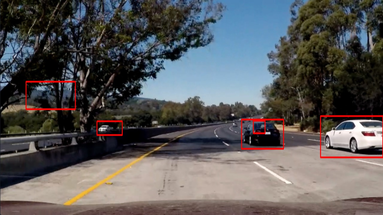
The image below shows mc.PLOT_PROB_THRESH = 0.5
Final thoughts
Reading through the paper was a real grind. Some math notations were a bit wonky; the paper referenced a lot and it was a recursive process. I literally had to crunch through the entire history of object detection to understand this paper. At the very least I hope you were able to get a high level understanding of this paper. Comment below with any corrections or questions!